The idea of a radio service ensuring coverage via transmitters operating on the same frequency is undoubtedly appealing. Beyond digital distribution methods, analog FM modulation also offers this possibility. Are single-frequency FM networks a new phenomenon destined to revolutionize FM band usage, or are they merely a solution born of necessity? This article aims to provide answers to these questions.

To set the stage, we will first present a few examples of single-frequency FM radio networks. Then, we will gradually move from theory to practice.

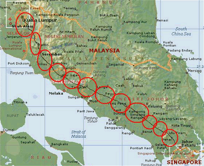
Fig. 1 – Example of a single-frequency FM network (highway radio).
Source: Single Frequency Networks. Broadcast Electronics Inc., 2008.

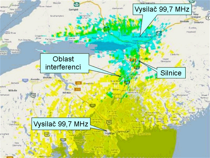
Fig. 2 – Example of a single-frequency network (rugged terrain).
Source: FM Single Frequency Networks. Nautel, 2015.

1. Single-frequency AM networks

It is worth taking a brief look at the past. The concept of analog broadcast networks where multiple transmitters operate on the same frequency is by no means new. Medium-wave AM transmitters were operating in this mode decades ago. The only significant requirement for such mode of operation was maintaining an absolutely identical carrier frequency across all transmitters; this was achieved for example using specialized receivers for the DCF77 time standard. GPS receivers with a synchronization frequency output serve this purpose just as well. You can use as many of these receivers as you like, place them wherever you wish, and they will all output the exact same frequency. This signal is fed into the AM transmitter's reference input, where the carrier frequency is derived from it using a phase-locked loop. Why is this important? Because even slightly different frequencies will interfere with each other at the receiver input, causing periodic signal fading or an audible heterodyne tone. The sound "swells" or whistles due to the difference between the carrier frequencies.

No special demands were placed on the processing and distribution of the modulation signal itself. Unlike FM, AM is classified as a linear modulation method because the principle of superposition applies to it. There is a linear relationship between the spectrum of the modulation signal and the spectrum of the resulting AM signal. Consequently, assuming equal signal strengths from the two transmitters, an AM receiver reproduces a simple sum (mix) of the transmitted audio. Occasionally, due to varying delays in distributing the modulation signal to the transmitters, an echo might occur during playback; a particularly proactive pensioner would then call the station to have it corrected — and that was essentially the extent of the issues that needed addressing.

2. Specifics of Single-Frequency FM Networks

What seemed straightforward with AM modulation is a real challenge with FM. While AM was forgiving of many things, FM is unforgiving. Let us admit right from the start that the result may not always be acceptable, even when everything is done perfectly. There are at least two reasons for this: FM is a non-linear modulation, and we generally want the audio to be stereophonic. The requirement for stereo sound is a particularly tough nut to crack. After all, single-frequency FM networks were historically considered exclusively for monophonic broadcasting — and there was a good reason for that. Yet, who today would be interested in broadcasting technology designed solely for mono operation? Marketing calls the shots, and the average modern listener is unconcerned with a loss in quality, so the technology is pushed to — and beyond — its limits.

From the perspective of detailed analysis, FM modulation is quite complex. Don't worry, we won't delve too deeply into that. However, we can briefly highlight a few interesting characteristics. For instance, a difference of just a few dB (typically cited as 3 to 4 dB) is enough for a stronger signal to overpower a weaker one. While this doesn't mean the receiver's audio output will be perfectly clean and interference-free — that would require a slightly larger margin — the content carried by the weaker signal becomes unrecognizable. Why is this insight important? Because we are analyzing the behavior of a single-frequency transmitter network. Clearly, the entire issue revolves around coverage areas where signals from multiple transmitters have similar levels. This is precisely where any potential negative effects manifest. In areas where one transmitter's signal is strongly dominant, there is effectively no simultaneous reception from multiple transmitters.

A single-frequency network can, of course, consist of a large number of transmitters. We will simplify things a bit: whenever we speak of a single-frequency network, we will be referring to a network of just two transmitters. There is still plenty to discuss, so you won't miss out on anything ;) In practice, this simplification works well, as signal overlap from more than two transmitters is something any sensible operator would avoid. Thus, even larger networks can be analyzed as separate pairs of transmitters.

2.1. Synchronous transmission in a single-frequency FM network

What happens when two signals with the same carrier frequency and equal signal strength arrive at the input of an FM receiver? While AM involves a simple summation (or even averaging, given the operating principle of a typical receiver) of the transmitted audio information, the situation with FM is unfortunately not so straightforward, as FM involves a non-linear process. We will therefore focus exclusively on FM transmission from this point on.

Fig. 3 – Linear (AM) and non-linear (FM) modulation, summation of modulated signals, and demodulated output.

In the case of FM, the resulting demodulated signal does indeed contain the original audio information fed into both modulators; however, the demodulation process also generates an additional component representing noise and distortion. The strength of this interfering component depends on the extent to which the modulating signals differed from one another at any given moment — and, crucially, the point relevant for assessing the alignment of the modulating signals is the reception site, not the transmitter modulation inputs. We will demonstrate in a moment why these two locations are not equivalent. To put it briefly and clearly: for an FM receiver to correctly reproduce a program received from multiple transmitters simultaneously — that is, to ensure listenability without unpleasant interference — there must be maximum alignment between the signals from the individual transmitters at the point of reception.

In practice, this means ensuring alignment of the

• carrier frequency
• time-domain characteristics of the MPX modulation signal — specifically the pilot tone, audio, and RDS
• frequency deviation — that is, the relationship between the instantaneous carrier frequency and the MPX signal waveform

If these conditions are met, we can speak of a synchronous network, synchronous operation, synchronous broadcasting, and so on.

Sometimes the term "synchronous broadcasting" is also used to describe situations where two transmitters broadcast the same program and sound subjectively identical, even though the conditions for true synchronous operation defined above are not fully met. One must be aware of this slight terminological ambiguity.

2.2. Effect of time delay

We established that for synchronous operation, the frequency deviation and the time profile of the modulation signal must match. However, signals propagate from transmitters at a finite speed — the speed of light. Clearly, a situation can arise where two originally identical signals arrive at the receiver with a relative time offset, depending on one's location. This disrupts the condition of signal alignment, causing an interference component to appear at the demodulator output. The result is audio distortion, increased noise, and degraded channel separation. This effect is identical to multipath propagation, where a mixture of direct and reflected signals strikes the antenna. The reflected signal carries the same audio information (the same modulation) but reaches the receiver input with a delay relative to the direct path. The greater the relative time offset between the signals and the smaller the difference in signal intensity, the more severe the interference effects become. Beyond a certain threshold, the audio becomes heavily distorted; in extreme cases, the reproduction is completely unintelligible.

As a rough guide, we can rely on experimental findings indicating that if both signals have equal intensity, a delay of up to 5 microseconds (µs) is barely acceptable; at this level, the interference is audible only in the background, and the stereo effect remains perceptible, albeit with significantly reduced separation. At a delay of 10 µs, a signal intensity difference of more than 6 dB is already required; at 15 µs, the difference must exceed 12 dB. If this difference is not maintained, the reproduction will exhibit severe distortion and significant interference (a "crackling" effect during modulation peaks).

If we are truly serious about listening quality and require a good signal-to-noise ratio and good channel separation, we should aim for a shorter delay in the overall design. We can base this, for example, on the phase difference of the stereo broadcast subcarrier, which has a frequency of 38 kHz. A reasonable criterion for maintaining acceptable listening quality is a stereo subcarrier phase difference of up to 30 degrees; such a difference corresponds to a relative delay of 2 µs. Let us examine what this situation looks like in terms of phase distribution along the signal propagation path.

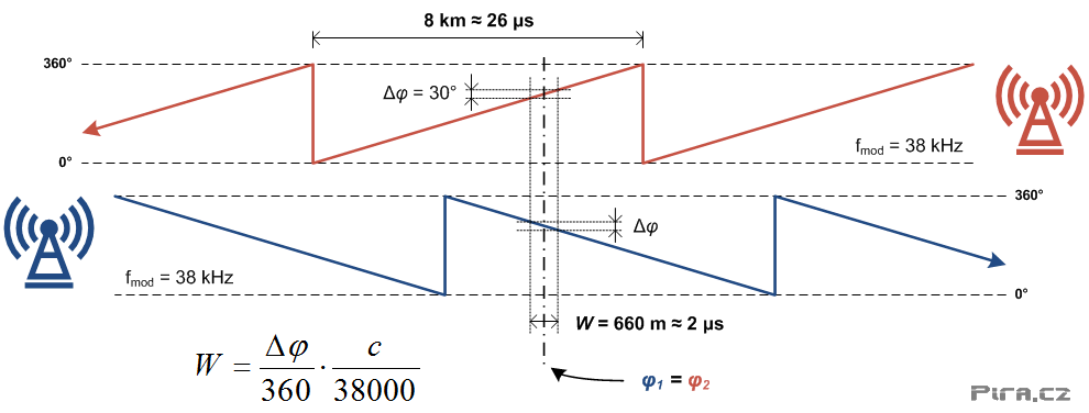
Fig. 4 – Instantaneous phase distribution of the 38 kHz subcarrier along the line connecting the transmitters, as a function of distance from the transmitters.

This figure is somewhat more complex; its purpose is to illustrate just how narrow the region actually is where signals from two transmitters meet in phase — or, more precisely, within the limits of the specified phase difference for the 38 kHz subcarrier. However, it is not always possible to precisely quantify the acceptable phase difference; this is a matter of subjective assessment based on local conditions and the program content. Ultimately, we must accept this, as the relationship is fixed, and only other network parameters can be altered.

To ensure high-quality listening in areas where signals from multiple transmitters mix at roughly equal intensities, the phase difference of the 38 kHz subcarrier must generally be kept within a range of a few tens of degrees. This implies, among other things, that synchronous reception along the line connecting two transmitters can only function reliably within a narrow strip a few hundred meters wide. These factors define the limitations of the single-frequency FM radio network concept. In short, these networks are not a full equivalent to single-frequency networks based on digital modulation.

3. Signal coverage of a single-frequency FM network

Based on the preceding information, we can now construct a basic diagram of signal coverage for a single-frequency network. The coverage area breaks down into several distinct zones.

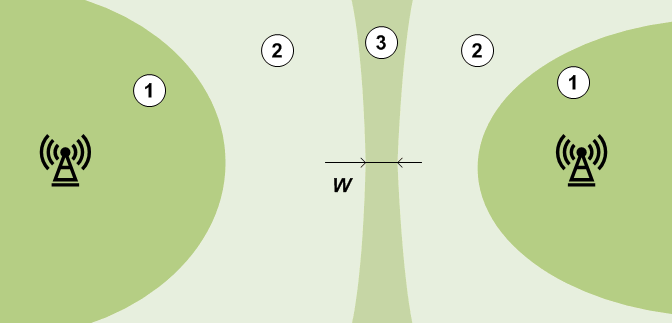
Fig. 5 - Schematic representation of coverage areas for a single-frequency transmitter network.
1 - Area with dominant signal strength from the nearest transmitter.
2 and 3 - Interference area.
3 - Synchronous reception area.
W: Width of the synchronous reception area – only a few hundred meters for stereo broadcasting.

We will now examine the individual areas in greater detail.

2.1. Area with dominant signal strength from the nearest transmitter

The name itself indicates how this area is characterized. As previously mentioned, reception in this coverage area is equivalent to receiving a signal from a single transmitter; consequently, there is no need to address the specific issues associated with a single-frequency network in this area.

In practice, it is desirable for this area to cover as much of the planned coverage zone as possible. Typically, this is an area with a direct line of sight to the nearest transmitter, while other transmitters in the network are either shielded by terrain or located at such a distance that their signals have no significant effect.

2.2. Interference Zone

An interference zone is an area where signals from multiple transmitters in a single-frequency network overlap. More precisely, it is an area where there is a certain minimum probability of a situation arising in which a receiver is exposed to comparable signal strengths from multiple transmitters. The word "probability" must be emphasized here. Whenever we speak of similar signal strengths, we are considering a specific receiver. This receiver has a specific antenna with specific directional characteristics and is located in an environment influenced by nearby obstacles. The area where interference between signals of similar levels can occur is usually more extensive than what the calculation software indicates. For instance, interference can occur even at a location where the calculation software predicts a 20 dB difference in signal strength. This can happen simply because a building stands in the path of the stronger signal — a scenario that calculation software typically does not account for.

The mutual interference of two signals naturally affects the strength of the received signal as well. This is worth noting because, even when the signals are perfectly aligned at the point of reception, we encounter another phenomenon: standing waves. In such a case, nodes and antinodes — representing minima and maxima of electromagnetic field intensity — alternate throughout the space. Where signals meet out of phase (carrier frequencies), the audio may degrade into noise. This is particularly noticeable when the receiver is in motion, as signal dropouts typically recur every few meters.

It is interesting to note that even in a synchronous transmission network, the alignment of carrier frequencies need not be absolutely perfect. Minor deviations or fluctuations are permissible, especially given the prevalence of mobile reception. After all, such reception is inevitably affected by the Doppler effect, meaning that perfect alignment would not occur at a moving receiver anyway.

The location and size of the interference zone can be modified by adjusting the placement and orientation of the transmitting antennas, as well as by changing the transmission power. The interference zone should ideally cover the smallest possible portion of the service area, since with analog FM modulation, there is no way to completely eliminate mutual interference in the resulting audio output. An ideal scenario, for instance, involves shielding two adjacent transmitters with a mountain ridge; this ensures a rapid transition from receiving one transmitter to the other, resulting in a very narrow interference zone. In such cases, a single-frequency network can effectively cover even relatively large areas.

2.3. Synchronous reception zone

The synchronous reception zone most often overlaps with the interference zone. It is the area where the relative delay between signals from two transmitters falls within a specified range — for example, up to 2 µs. Naturally, the aim is to position the synchronous reception zone where there is the highest probability of the receiver being exposed to signals of comparable strength from multiple transmitters.

It follows that in a single-frequency network, the relative delay of signals from individual transmitters must be controlled — that is, preset. Of course, the listener coverage in the given area must also be taken into account during this process. It makes no sense to position the synchronous reception zone in areas with rocks, forests, or fields; instead, it should be located where the highest concentration of receivers is expected. Determining the setup often involves a compromise. Outside the synchronous reception zone, one must anticipate a significant drop in listening quality if signals from multiple transmitters reach the receiver input at comparable levels. The synchronous reception zone is narrowest along the line connecting the transmitters, as the signals there are propagating directly towards each other.

4. Technical implementation of a single-frequency FM network

A single-frequency network can be implemented using purely analog FM transmitters or transmitters that generate the FM signal via digital signal processing techniques — typically DDS (Direct Digital Synthesis). Naturally, the two approaches differ in certain details, particularly regarding the adjustment of parameters to specific conditions.

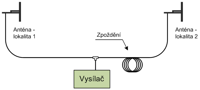
Fig. 6 – Principle of a single-frequency FM network.

The figure above illustrates the intended outcome. Each antenna is located at a different transmission site; the difference in cable lengths determines the relative delay and, consequently, the position of the synchronous reception zone. While the technical solution shown here is functional, it is also extremely "hardcore," as it would require laying potentially tens of kilometers of coaxial cable. All practical solutions seek a way to avoid such an approach. This entails using separate FM transmitters operated in synchronous mode.

4.1. Analog solution

Several analog solutions were developed in the past, though their significance today is minimal. We will briefly describe one possible approach.

Analog devices are characterized, among other things, by the fact that no two units are completely identical. With standard FM transmitters, ensuring perfect matching of the output FM signal would be highly problematic. Every analog FM modulator exhibits certain deviations — whether in sensitivity (frequency dependence on input voltage), linearity, frequency response, step response, etc. For this reason, the entire network uses a single shared FM modulator. Its output signal must be distributed to the individual transmitters. There, using a mixer and a precision GPS-controlled oscillator, the signal is converted to the required frequency within the FM broadcast band. In practice, this is slightly more complex due to the need for filtering, but this issue can be eliminated through appropriate techniques. A purely analog solution naturally presents difficulties regarding the adjustment of signal time delays at individual transmitters — or, more precisely, it does not allow for such adjustment at all. The delay is fixed and determined by the distances from the modulator to the individual transmitters.

A synchronous signal repeater serves as an example of an analog solution. We cannot simply take a radio signal, amplify it, and immediately re-transmit it via an antenna on the same frequency, because the output signal would feed back into the input, causing the entire system to oscillate. Therefore, the repeater's input must be located far enough away to avoid interference from the output.

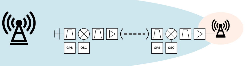
Fig. 7 - Analog synchronous repeater.

Therefore, near the primary transmitter, we shift the signal to a different carrier frequency using a mixer and a GPS-controlled oscillator. We perform the reverse process at the repeater and can then transmit the amplified signal. The output signal delay is virtually identical to the delay of the signal from the primary transmitter; the repeater is thus located directly within the synchronous reception zone and can operate at low power. This is a somewhat simplified explanation, but the concept is clear, and it suffices for the scope of this article.

4.2. Digital solution

A digital FM transmitter based on the DDS principle offers full control over FM modulation, as the modulation is generated via calculation. Consequently, the FM modulator can be an integral part of each transmitter. The modulation signal is delivered to them in digital form — for example, via the Internet or a dedicated data line. Since this method of signal delivery often entails unpredictable latency, the transmitters must be synchronized in some way. Simply put, the incoming data stream contains timestamps alongside the MPX signal samples; the data is stored in a buffer at the transmitter and, upon receiving a command in the form of a common synchronization pulse, leaves the buffer to proceed directly to the modulator. The aforementioned time stamps ensure that, at any given moment, the modulation signal enters the modulator at all transmitters at a specific time position (represented by a specific sample). The source of the synchronization pulses is — naturally — GPS receivers, with their output designated as 1PPS (1 pulse per second). The timing alignment of these pulses is accurate to within nanoseconds, which also represents the theoretical precision for setting the delay at individual transmitters (in practice, such high precision is not available, nor is it required).

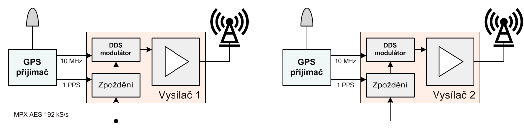
Fig. 8 – Digital solution for a single-frequency FM network.

By adjusting the signal delay at the transmitter, the synchronous reception zone can be positioned with an accuracy of tens or hundreds of meters. The technology itself imposes no limitations in this regard. However, as we have seen, determining where this zone should actually be located often presents a challenge. Given its limited width, the setting is essentially a matter of compromise — which an optimist might view as a solution that satisfies everyone, while a realist might argue that a compromise is a solution that satisfies no one. Today, manufacturers offer equipment that places no restrictions on broadcasters; the limitations are inherent to the FM broadcasting principle itself. How each operator handles this is entirely up to them. Manufacturers are quick to point out that they do not provide consulting services in this area. In essence, they are saying: "Here is the hardware — theoretically capable of anything — now figure out how to use it yourself." A thorough analysis and design of the single-frequency network, combined with experimental verification, are essential prerequisites for successful future operation and help prevent potential disappointment with actual results.

5. Conclusion

Single-frequency FM networks enable more efficient use of the radio spectrum — thereby reducing the number of frequencies required — and, in certain respects, simplify receiver operation. However, their implementation is practical only in a relatively small number of specific cases. A reduction in reproduction quality invariably occurs in areas of overlap. Economic considerations also act as a limiting factor — specifically, the cost of the design and technology relative to the size and economic importance of the area being covered.

Author: Ing. Jan Kolar